Chebyshev Polynomials
The Chebyshev Polynomials are two sequences of polynomials that are of primal importance in numerical analysis. Chebyshev polynomials are often used to approximate functions due to their optimality in minimizing the approximation error. When a function is approximated by a Chebyshev series, the error tends to oscillate evenly between positive and negative values, minimizing the worst-case error (the Chebyshev equioscillation theorem).
- The Chebyshev polynomials of the first kind \(T_n(x)\);
- The Chebyshev polynomials of the second kind \(U_n(x)\).
where
\[T_{n+1}(x) = 2x T_n(x) - T_{n-1}(x)\quad T_0(x) = 1, T_1(x) = x \\ U_{n+1}(x) = 2x U_n(x) - U_{n-1}(x)\quad U_0(x)=1, U_1(x) = 2x.\]These are related to trigonometric functions, as
\[T_n(\cos\theta) = \cos(n\theta)\\ U_n(\cos\theta)\sin\theta = \sin\left((n+1)\theta\right).\]This suggests that the \(k\)th Chebyshev polynomial of the first kind can be defined as the real part of the function \(z^k\) on the unit circle,
\[T_k(x) = \text{Re}(z^k) = \frac{1}{2}(z^k+ z^{-k}) = \cos(k\theta).\]WIth respect to the following inner product the \(T_n(x)\)s are orthogonal to each other,
\[\langle f,g\rangle = \int_{-1}^1 f(x) g(x)\frac{dx}{\sqrt{1-x^2}},\]so that
\[\langle T_n, T_m\rangle =\begin{cases} 0 & n\neq m \\ \pi & n=m=0 \\ \frac{\pi}{2} & n=m\neq 0\end{cases}.\]Similarly, for \(U_n\),
\[\int_{-1}^1 U_n(x) U_m(x) \sqrt{1-x^2} dx = \begin{cases} 0 & n\neq m \\ \frac{\pi}{2} & n=m \end{cases}.\]Chebyshev series#
Theorem. If \(f\) is Lipschitz continuous on \([-1,1]\), it has a unique representation as a Chebyshev series,
\[f(x) = \sum_{k=0}^{\infty} a_k T_k(x)\]which is absolutely and uniformly convergent, and where
\[a_k = \frac{2}{\pi} \int_{-1}^1 \frac{f(x)T_k(x)}{\sqrt{1-x^2}}dx,\]and for \(k=0\) by the same formula with the factor being \(1/\pi\).
(Recall that Lipschitz continuity means there is a constant \(C\) s.t. \(|f(x)-f(y)| < C|x-y|\) for all \(x,y\in[-1,1]\).)
Chebyshev Points#
We have \(n\)th roots of unity \(z_n = e^{2\pi i/n}\). Consider the multiples of (2\(n\))th roots of unity \(z_j = e^{i\pi /n}, -n+1\leq j \leq n\) instead. These corresponds to the Chebyshev points \(x_j =\cos(j\pi/n), 0\leq j \leq n\), and also to the equispaced points \(\theta_j = j\pi/n, -n+1\leq j \leq n\) in \([-\pi,\pi]\).
\(T_k\) takes alternating values \(\pm 1\) at the \(k+1\) Chebyshev points\(\(.\)
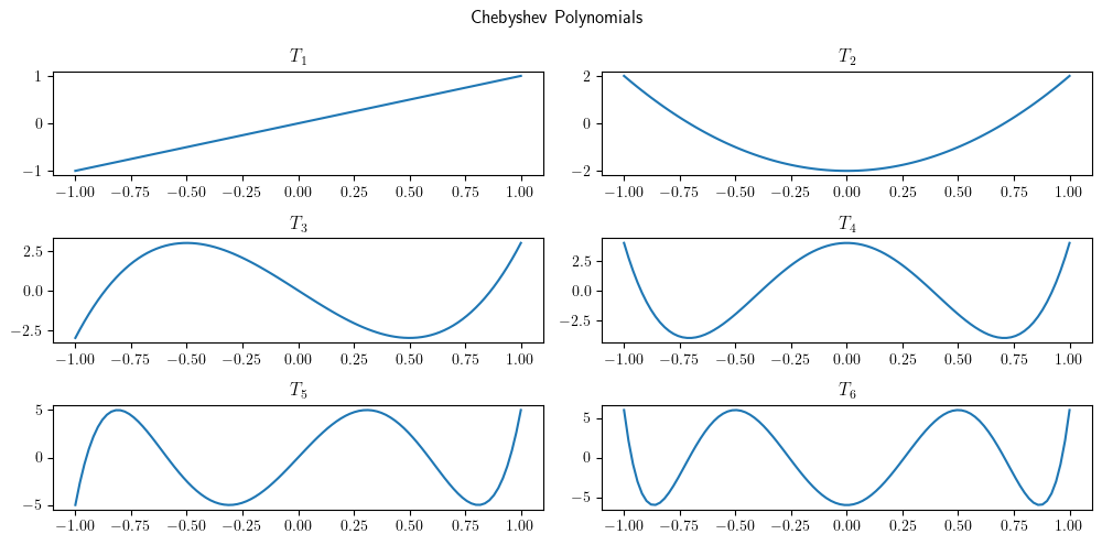
First few Chebyshev Polynomials#
import numpy as np
import matplotlib.pyplot as plt
plt.rcParams['text.usetex'] = True

fig, axs = plt.subplots(3,2,figsize=(10,5))
xs = np.linspace(-1,1,100)
for j in range(2):
    for i in range(3):
        axs[i][j].plot(xs,np.polynomial.chebyshev.Chebyshev.basis(i*2+j+1)(xs))
        axs[i][j].set_title(r'T_{}'.format(i*2+j+1))
fig.suptitle('Chebyshev Polynomials')
fig.tight_layout()
The Chebyshev points are the extremes of each curve.
Chebyshev, Laurent, Fourier#
There are three closely analogous canonical settings asosciated with the names of Fourier, Laurent, and Chebyshev. The Chebyshev setting concerns a variable \(x\) and a function \(f\) defined on \([-1,1]\):
\[x\in [-1,1],\quad f(x)\approx \sum_{k=0}^n a_k T_k(x).\]Let \(z\) be a variable that ranges over the unit circle in the complex plane, i.e. \(|z| =1, z\in \mathbb{C}\). Put \(F(x) = f(x)\) where \(x=(z+z^{-1})/2\) - there are two values of \(z\) for each value of \(x\) and \(F\) satisfies \(F(z)= F(z^{-1})\) and the series now involves a polynomial in both \(z\) and \(z^{-1}\) known as a Laurent polynomial:
\[|z|=1, \quad F(z) = F(z^{-1}) \approx \frac{1}{2}\sum_{k=0}^n a_k(z^k+z^{-k}).\]Now let \(\theta \in [-\pi,\pi]\), put \(\mathcal{F}(\theta) = F(e^{i\theta}) = f(\cos(\theta))\), then there is a 1-to-1 correspondence \(z = e^{i\theta}\) and a 2-to-1 correspondence between \(\theta\) and \(x\) with \(\mathcal{F}(\theta)=\mathcal{F}(-\theta)\). The series is now a Fourier polynomial:
\[\theta\in[-\pi,\pi],\quad \mathcal{F}(\theta) = \mathcal{F}(-\theta) \approx\frac{1}{2}\sum_{k=0}^n a_k(e^{ik\theta}+e^{-ik\theta}).\]Example#
The chebyshev approximation of \(\sin(6x) + \sin(60e^x)\) is as follows:
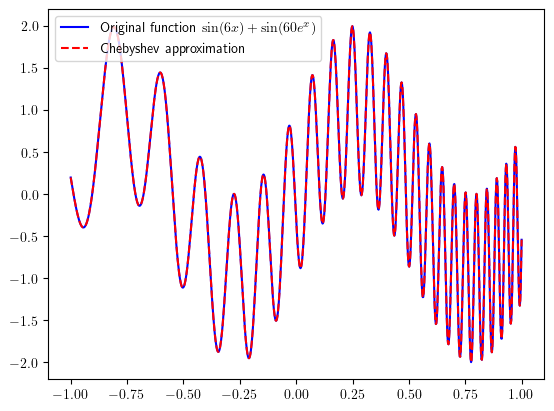 | 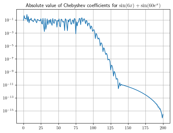 |
We see that up to degree about \(k=100\) a Chebyshev series cannot resolve the function \(f\) much; the oscillation occurs at short wave lengths. After that the series converges rapidly.
def f(x):
    return np.sin(6*x) + np.sin(60*np.exp(x))

degree = 200

x = np.linspace(-1, 1, 1000)

coeffs = np.polynomial.chebyshev.chebfit(x, f(x), degree)

f_reconstructed = np.polynomial.chebyshev.chebval(x, coeffs)

plt.plot(x, f(x), label=r'Original function $\sin(6x) +\sin60(e^x)$', color='blue')
plt.plot(x, f_reconstructed, label='Chebyshev approximation', linestyle='dashed', color='red')
plt.legend()
plt.show()
fig, ax = plt.subplots()
ax.plot(range(degree+1), abs(coeffs))
ax.grid(True)
ax.set_yscale('log')
ax.set_title(r'Absolute value of Chebyshev coefficients for $\sin(6x) +\sin60(e^x)$')
plt.show()